Adanced Fitting
This section describes how to use advanced features of fitterpp.
The section assumes that you have read the
basic tutorial. Specifically, you should be
familiar with the following the calcParabola function
we used as an example of fitting
def calcParabola(center=None, mult=None, xvalues=XVALUES):
    estimates = np.array([mult*(n - center)**2 + for n in xvalues])
    return pd.DataFrame({"x": xvalues, "y": estimates})
and the following script that fits the observational data data_df
to the parameters center and mult in calcParabola.
# Import the required libraries
import lmfit
import fitterpp as fpp
# Construct the parameter objects
parameters = lmfit.Parameters()
parameters.add("center", value=0, min=0, max=100)
parameters.add("mult", value=0, min=0, max=100)
# Run the fitting algorithm
fitter = fpp.Fitterpp(calcParabola, parameters, data_df)
fitter.execute()
# Display the fittted values
print(fitter.final_params.valuesdict())
A first consideration in more advanced fitting is to have more
control over the way in which fitterpp searches for parameter
values.
This is accompished by making use of an optional keyword parameter
in the constructor, fpp.Fitterpp.
You can specify any algorithm that is used by lmfit.minmize.
To simplify common usage, fitterpp provides global constants
for the “leastsq” and “differential_evolution” algorithms.
# Spsecify the methods used for fitting
methods = fpp.Fitterpp.mkFitterMethod(
      method_names=fpp.METHOD_DIFFERENTIAL_EVOLUTION,
      method_kwargs={fpp.MAX_NFEV: 1000})
fitter = fpp.Fitterpp(calcParabola, parameters, data_df,
      methods=methods)
A second consideration in more advanced fitting is the tradeoff between the followin: * quality of the fit and * runtime of the fitting codes.
Runtime of the fitting codes is typically measured in seconds. We quantify the quality of the fit by the sum of squares of the residuals or RSSQ. If there is a perfect match between the observational data and the estimates produced by fitted parameters, then RSSQ is 0. Larger values of RSSQ indicate a fit that with lower quality. Many times a fitting problem involves trade-offs between quality and runtime.
You can get a basic understanding of the quality of the fit
from the fitter report.
Building on the example in the basic tutorial,
As before, we are fitting the parameters of calcParabola.
To use this feature, first perform a fit and then use
print(fitter.report())
This produces the output below:
[[Variables]]
    mult:  2.0102880244080366
    center:  10.000857728276536
[[Fit Statistics]]
    # fitting method   = differential_evolution
    # function evals   = 921
    # data points      = 20
    # variables        = 2
    chi-square         = 2.54104032
    reduced chi-square = 0.14116891
    Akaike info crit   = -37.2631740
    Bayesian info crit = -35.2717095
Of most interest here is the number of function evalutions–921. This provides some insight into the extent of the search for fitting values.
The quality plot indicates how RSSQ changes across iterations. Sometimes, a large fraction of iterations do not result in reductions in RSSQ. To generate the quality plot use:
fitter.plotQuality()
which produces the plot
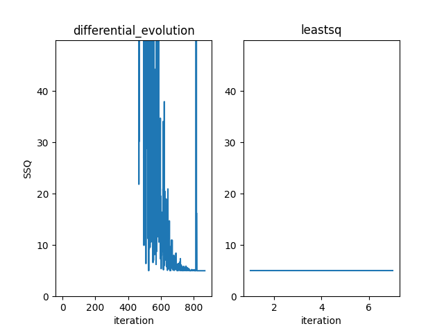
Note that the y-axis of the plot is scaled to show RSSQ values within ten times the minimal RSSQ. From this plot, we observe that (a) differential evolution rquires about 800 iterations before RSSQ is reduced substantially; and (b) gradient descent (“leastsq”) provides little reduction in RSSQ.
Finally, the performance plot provides insight into the causes of long runtimes. To generate the performance plot use:
fitter.plotPerformance()
which produces the plot below.
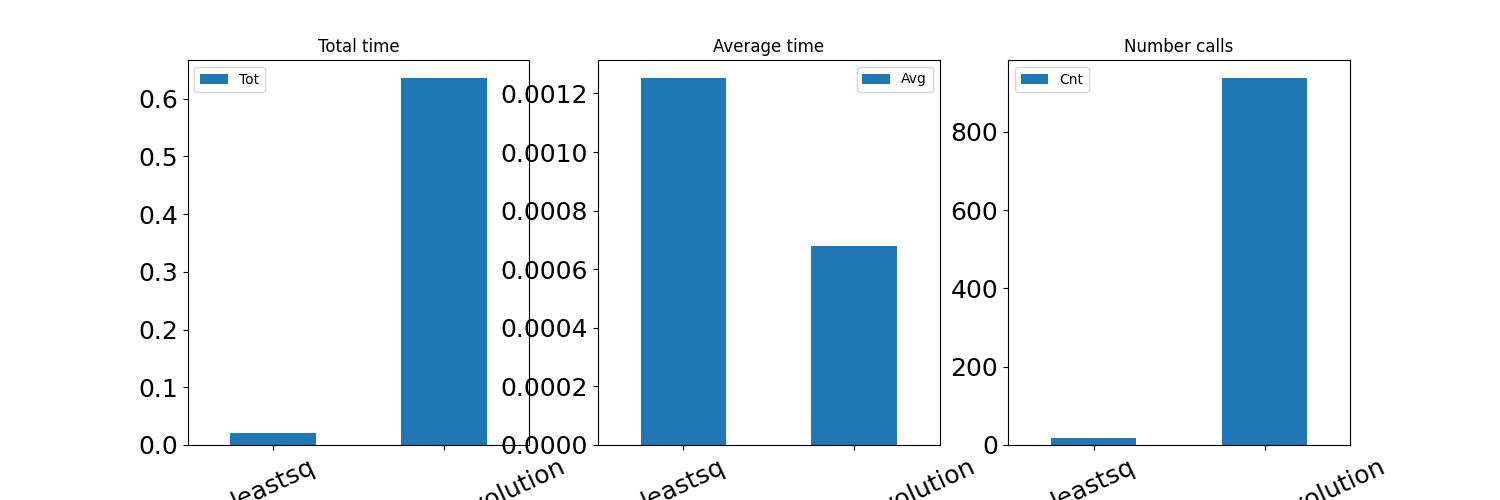
From this we conclude that the time required to fit the parameters is large due to the large number of iterations of differential evolution.